Contents
The Generalized Beamformer: All Transmit Sequence Types
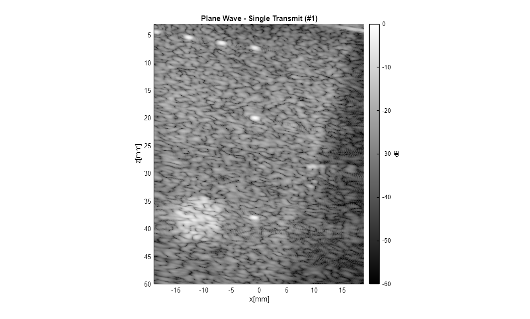
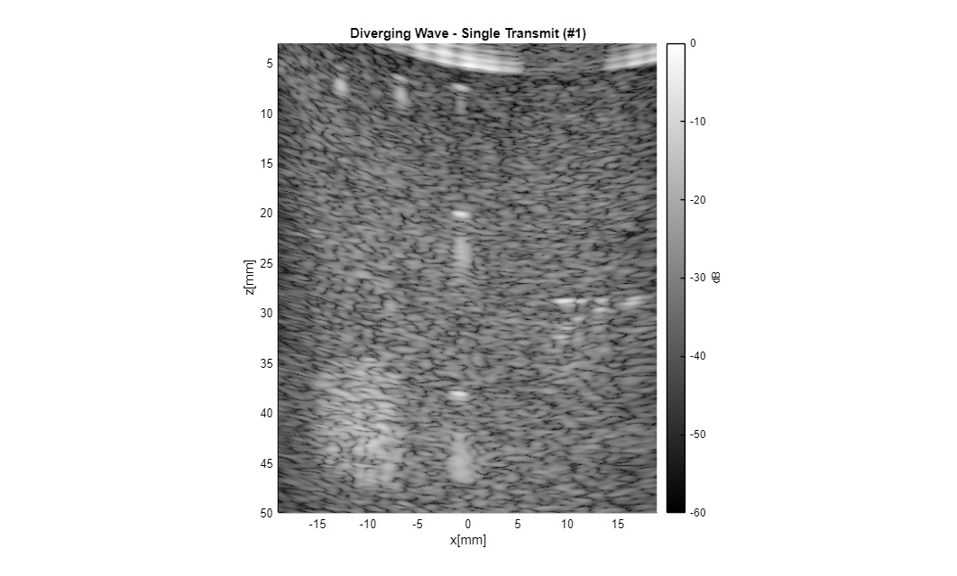
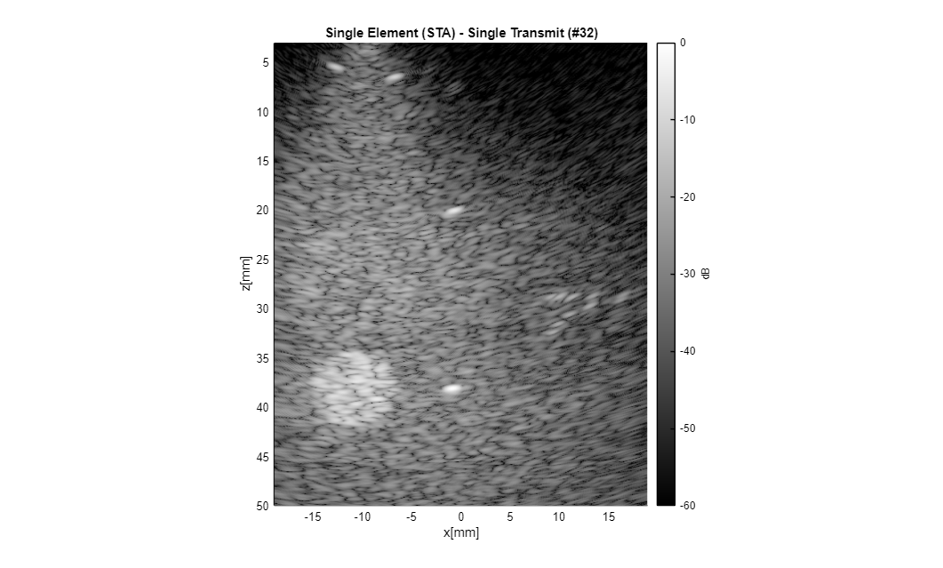
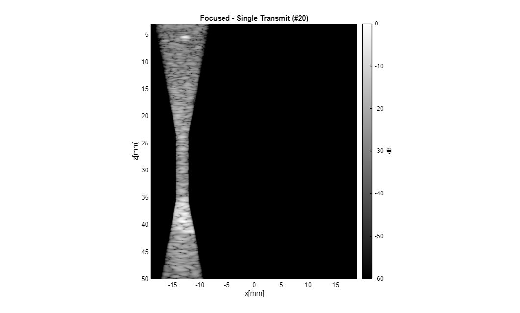
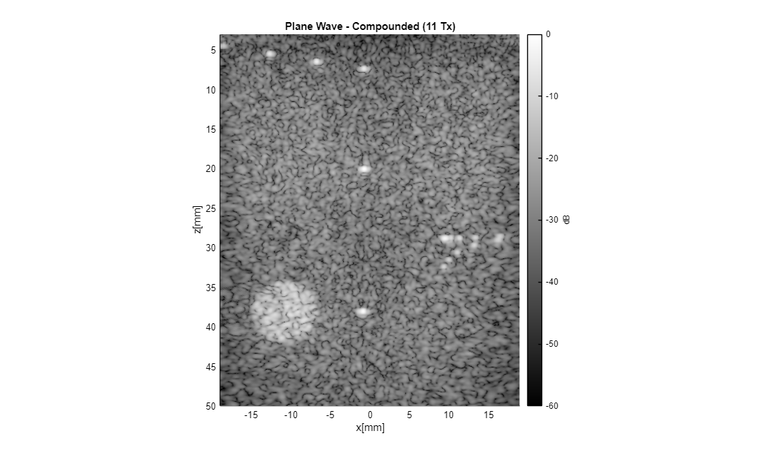
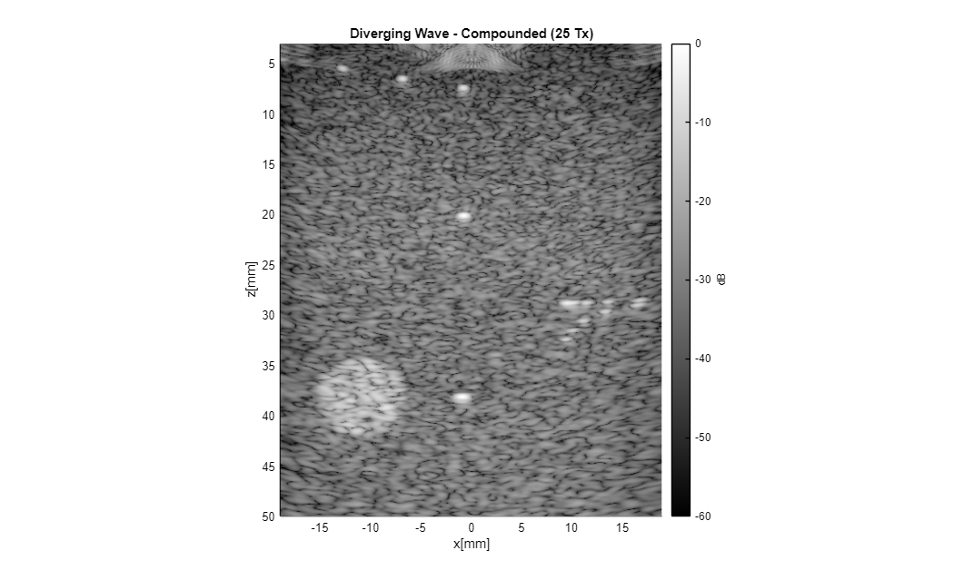
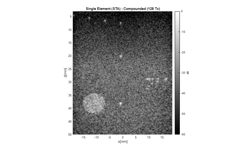
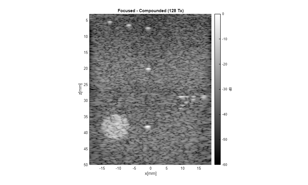
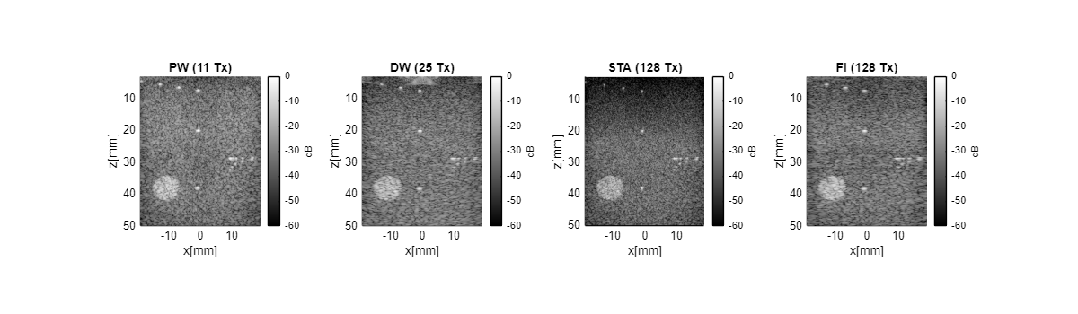
This example demonstrates the Generalized Beamformer (GB) from the UltraSound ToolBox (USTB). A single beamforming equation handles four fundamentally different transmit sequences: plane wave, diverging wave, single-element (STA), and focused imaging. Only the transmit delay model and apodization parameters change between them.
The results correspond to Figure 5 in: Rindal et al., "The Generalized Beamformer in the UltraSound ToolBox", Ultrasonics, 2026.
by Ole Marius Hoel Rindal olemarius@olemarius.net
clear all;
close all;
if strcmp(tools.headless_publish_figure_visible(), 'on')
    set(groot, 'DefaultFigureVisible', 'on');
end
Dataset definitions
All four datasets were acquired on a Verasonics Vantage 256 using a Philips L7-4 linear array (128 elements, 0.298 mm pitch, ~5.2 MHz center frequency) and a CIRS 054GS phantom. The received channel data were sampled at 20.8 MHz (4x center frequency).
url = tools.zenodo_dataset_files_base();

all_filenames{1} = 'L7_CPWC_TheGB.uff'; selected_tx(1) = 1;  tag{1} = 'PW';  tag_title{1} = 'Plane Wave';
all_filenames{2} = 'L7_DW_TheGB.uff';   selected_tx(2) = 1;  tag{2} = 'DW';  tag_title{2} = 'Diverging Wave';
all_filenames{3} = 'L7_STA_TheGB.uff';  selected_tx(3) = 32; tag{3} = 'STA'; tag_title{3} = 'Single Element (STA)';
all_filenames{4} = 'L7_FI_TheGB.uff';   selected_tx(4) = 20; tag{4} = 'FI';  tag_title{4} = 'Focused';

dynamic_range = 60;
Download and beamform all four transmit types
Each dataset is beamformed using the GB in USTB (midprocess.das). The only difference between the four is the transmit apodization and delay model configuration. A constant f-number expanding receive aperture with a Hamming window is used throughout.
for f = 1:length(all_filenames)
    filename = all_filenames{f};
    tools.download(filename, url, data_path);
    channel_data = uff.read_object([data_path filesep filename], '/channel_data');
    channel_data.N_frames = 1;

    if contains(filename, 'DW') || contains(filename, 'FI')
        for seq = 1:channel_data.N_waves
            channel_data.sequence(seq).sound_speed = channel_data.sound_speed;
        end
    end

    scan = uff.linear_scan();
    scan.x_axis = linspace(channel_data.probe.x(1), channel_data.probe.x(end), 512).';
    scan.z_axis = linspace(3e-3, 50e-3, 512).';
UFF: reading channel_data [uff.channel_data]
UFF: reading sequence [uff.wave] [====================] 100%
Warning: You just deleted all frames except frames 1 to 1, I hope you meant to!
UFF: reading channel_data [uff.channel_data]
UFF: reading sequence [uff.wave] [====================] 100%
Warning: You just deleted all frames except frames 1 to 1, I hope you meant to!
UFF: reading channel_data [uff.channel_data]
UFF: reading sequence [uff.wave] [====================] 100%
Warning: You just deleted all frames except frames 1 to 1, I hope you meant to!
UFF: reading channel_data [uff.channel_data]
UFF: reading sequence [uff.wave] [====================] 100%
Warning: You just deleted all frames except frames 1 to 1, I hope you meant to!
Set up the Generalized Beamformer
    mid = midprocess.das();
    mid.dimension = dimension.receive;
    mid.channel_data = channel_data;
    mid.scan = scan;

    if contains(filename, 'FI')
        MLA = scan.N_x_axis / channel_data.N_waves;
        mid.spherical_transmit_delay_model = spherical_transmit_delay_model.hybrid;
        mid.pw_margin = 2/1000;
        mid.transmit_apodization.window = uff.window.tukey25;
        mid.transmit_apodization.f_number = 2.5;
        mid.transmit_apodization.MLA = MLA;
        mid.transmit_apodization.MLA_overlap = MLA;
        mid.transmit_apodization.minimum_aperture = [2.5e-03 2.5e-03];
    else
        mid.transmit_apodization.window = uff.window.none;
        mid.transmit_apodization.f_number = 1.7;
    end

    mid.receive_apodization.window = uff.window.hamming;
    mid.receive_apodization.f_number = 1.7;

    fprintf('\n=== Beamforming: %s (%d transmits) ===\n', tag_title{f}, channel_data.N_waves);
    b_data_single_tx = mid.go();

    b_data = uff.beamformed_data(b_data_single_tx);
    b_data.data = reshape(b_data.data, size(b_data.data,1), 1, 1, size(b_data.data,3));
=== Beamforming: Plane Wave (11 transmits) ===
USTB MEX C beamformer...Completed in 2.05 seconds.
=== Beamforming: Diverging Wave (25 transmits) ===
USTB MEX C beamformer...Completed in 3.29 seconds.
=== Beamforming: Single Element (STA) (128 transmits) ===
USTB MEX C beamformer...Completed in 24.52 seconds.
=== Beamforming: Focused (128 transmits) ===
USTB MEX C beamformer...Completed in 2.19 seconds.
Single transmit image
Showing a single transmit event before coherent compounding. This illustrates the raw contribution of one transmit to the final image.
    b_data_tx = uff.beamformed_data(b_data);
    b_data_tx.data = b_data.data(:, 1, 1, selected_tx(f));
    tools.publish_beamformed_snap(b_data_tx, ...
        sprintf('%s - Single Transmit (#%d)', tag_title{f}, selected_tx(f)), ...
        dynamic_range, 'log');
Coherent compounding
All transmit events are coherently summed to produce the final high-quality image. The GB handles this identically for all four transmit types.
    cc = postprocess.coherent_compounding();
    cc.input = b_data_single_tx;
    b_data_CC = cc.go();

    if contains(filename, 'FI')
        tx_comp = sum(mid.transmit_apodization.data, 2);
        b_data_CC.data = b_data_CC.data .* (1./tx_comp);
    end

    tools.publish_beamformed_snap(b_data_CC, ...
        sprintf('%s - Compounded (%d Tx)', tag_title{f}, channel_data.N_waves), ...
        dynamic_range, 'log');

    img_single{f} = b_data;
    img_compound{f} = b_data_CC;
    n_tx(f) = channel_data.N_waves;
end
Summary: All compounded images
The four compounded images are shown side by side. Despite using fundamentally different transmit wavefronts (plane, diverging, single element, focused), the Generalized Beamformer produces comparable image quality for all — demonstrating the unified nature of the approach.
f_all = figure('Position', [100 100 1200 350]);
for i = 1:4
    img_compound{i}.plot(subplot(1,4,i), ...
        sprintf('%s (%d Tx)', tag{i}, n_tx(i)), dynamic_range);
end
set(f_all, 'Color', 'w');
tools.publish_snap_now_figure(f_all);
Acquisition parameters
The table below summarizes the key acquisition parameters for each transmit sequence type.
fprintf('\n=== Acquisition Parameters ===\n');
fprintf('%-12s  %8s  %12s  %8s\n', 'Type', 'N_Tx', 'fs (MHz)', 'Elements');
fprintf('%s\n', repmat('-', 1, 50));
for i = 1:4
    fprintf('%-12s  %8d  %12.4f  %8d\n', tag{i}, n_tx(i), 20.8333, 128);
end
fprintf('\nAll sequences use f#=1.7 receive, Hamming window, 60 dB dynamic range.\n');
=== Acquisition Parameters ===
Type              N_Tx      fs (MHz)  Elements
--------------------------------------------------
PW                  11       20.8333       128
DW                  25       20.8333       128
STA                128       20.8333       128
FI                 128       20.8333       128

All sequences use f#=1.7 receive, Hamming window, 60 dB dynamic range.