Contents

CPWC Double Adaptive Beamforming - Explicit Processing (No Pipeline)

This script performs double adaptive beamforming using Capon Minimum Variance (MV) beamforming. It uses explicit midprocess/postprocess calls instead of the pipeline feature - the conventional way of doing processing in USTB.

Five different beamforming configurations are compared: 1. DAS on RX -> DAS on TX (Conventional) 2. MV on RX -> DAS on TX 3. DAS on RX -> MV on TX 4. MV on RX -> MV on TX (Double Adaptive) 5. DAS on TX -> MV on RX

Author: Ole Marius Hoel Rindal olemarius@olemarius.net

clear all;
close all;

Download and load channel data

url = 'http://ustb.no/datasets/';
filename = 'PICMUS_numerical_calib_v2.uff';

tools.download(filename, url, data_path);

channel_data = uff.channel_data();
channel_data.read([data_path, filesep, filename], '/channel_data');

UFF: reading /channel_data [uff.channel_data]
UFF: reading sequence [uff.wave] [====================] 100%

Define scan

scan = uff.linear_scan('x_axis', linspace(-20e-3, 20e-3, 256).', ...
                       'z_axis', linspace(10e-3, 50e-3, 256).');
%scan = uff.linear_scan('x_axis', linspace(-20e-3, 20e-3, 768).', ...
%                       'z_axis', linspace(10e-3, 50e-3, 512).');
%scan=uff.linear_scan('x_axis',linspace(0e-3,15e-3,256).', 'z_axis', linspace(23e-3,27e-3,256).');

Create apodization objects

Transmit apodization

transmit_apodization = uff.apodization();
transmit_apodization.probe = channel_data.probe;
transmit_apodization.sequence = channel_data.sequence;
transmit_apodization.focus = scan;
transmit_apodization.window = uff.window.tukey75;
transmit_apodization.minimum_aperture = [3.07000e-03 3.07000e-03];
transmit_apodization.f_number = 1.75;
transmit_apodization_with_window = transmit_apodization;

% Receive apodization
receive_apodization = uff.apodization();
receive_apodization.probe = channel_data.probe;
receive_apodization.focus = scan;
receive_apodization.window = uff.window.tukey25;
receive_apodization.f_number = 1.75;

% Receive apodization for MV on tx
receive_apodization_none_window = uff.apodization();
receive_apodization_none_window.probe = channel_data.probe;
receive_apodization_none_window.focus = scan;
receive_apodization_none_window.window = uff.window.none;

% Pre-compute apodization data (so it doesn't affect timing)
transmit_apodization.data;
receive_apodization.data;
receive_apodization_none_window.data;

Create midprocess DAS object

das = midprocess.das();
das.channel_data = channel_data;
das.scan = scan;
das.transmit_apodization = transmit_apodization;
das.receive_apodization = receive_apodization;

Configure Capon Minimum Variance beamformers

Receive adaptive (Capon MV)

adapt_rx = postprocess.capon_minimum_variance();
adapt_rx.dimension = dimension.receive;
adapt_rx.scan = scan;
adapt_rx.channel_data = channel_data;
adapt_rx.K_in_lambda = 1.5;
adapt_rx.L_elements = floor(channel_data.probe.N_elements/2);
adapt_rx.regCoef = 1/100;
adapt_rx.transmit_apodization = transmit_apodization;
adapt_rx.receive_apodization = receive_apodization;



% Transmit adaptive (Capon MV)
adapt_tx = postprocess.capon_minimum_variance();
adapt_tx.dimension = dimension.transmit;
adapt_tx.scan = scan;
adapt_tx.channel_data = channel_data;
adapt_tx.K_in_lambda = 1.5;
adapt_tx.L_elements = channel_data.probe.N_elements;
adapt_tx.regCoef = 1/100;
adapt_tx.transmit_apodization = transmit_apodization;
adapt_tx.receive_apodization = receive_apodization;

% Display settings
compression = 'log';
dynamic_range = 60;

=========================================================================

IMAGE 1: DAS on RX -> DAS on TX : Conventional

=========================================================================

fprintf('\n=== Processing Image 1: Conventional DAS ===\n');

das.transmit_apodization = transmit_apodization;
transmit_apodization.data;
das.dimension = dimension.both;

tic();
img{1} = das.go();
time{1} = toc();

label{1} = 'DASonRX->DASonTX';
fprintf('Completed in %.2f seconds.\n', time{1});
img{1}.plot()

=== Processing Image 1: Conventional DAS ===
USTB MEX C beamformer...Completed in 0.11 seconds.
Completed in 0.12 seconds.

ans = 

  Figure (1) with properties:

      Number: 1
        Name: ''
       Color: [1 1 1]
    Position: [232 146 560 420]
       Units: 'pixels'

  Use GET to show all properties

=========================================================================

IMAGE 2: MV on RX -> DAS on TX

=========================================================================

fprintf('\n=== Processing Image 2: MV on RX -> DAS on TX ===\n');

% Step 1: DAS with no compounding (dimension.none)
das.dimension = dimension.none;
das.transmit_apodization = transmit_apodization;

% Update adapt_rx parameters
adapt_rx.L_elements = floor(2*channel_data.probe.N_elements/3);
adapt_rx.regCoef = 1/100;

tic();
b_data_das = das.go();

% Step 2: Apply adaptive RX beamforming
adapt_rx.input = b_data_das;
b_data_adapt_rx = adapt_rx.go();
%
% Step 3: Coherent compounding on TX dimension
das_tx = postprocess.coherent_compounding();
das_tx.dimension = dimension.transmit;
das_tx.receive_apodization = receive_apodization;
das_tx.transmit_apodization = transmit_apodization_with_window;
das_tx.input = b_data_adapt_rx;
img{2} = das_tx.go();

time{2} = toc();

label{2} = 'MVonRX->DASonTX';
fprintf('Completed in %.2f seconds.\n', time{2});
img{2}.plot()

=== Processing Image 2: MV on RX -> DAS on TX ===
USTB MEX C beamformer...Completed in 0.24 seconds.
Completed in 34.92 seconds.

ans = 

  Figure (2) with properties:

      Number: 2
        Name: ''
       Color: [1 1 1]
    Position: [232 146 560 420]
       Units: 'pixels'

  Use GET to show all properties

=========================================================================

IMAGE 3: DAS on RX -> MV on TX

=========================================================================

fprintf('\n=== Processing Image 3: DAS on RX -> MV on TX ===\n');

% Update adapt_tx parameters
adapt_tx.L_elements = floor(channel_data.N_waves/3);
adapt_tx.regCoef = 1/100;
adapt_tx.receive_apodization = receive_apodization;

% Step 1: DAS on receive only
das.dimension = dimension.receive;
das.receive_apodization = receive_apodization;

tic();
b_data_das = das.go();

% Step 2: Apply adaptive TX beamforming
adapt_tx.input = b_data_das;
img{3} = adapt_tx.go();

time{3} = toc();

label{3} = 'DASonRX->MVonTX';
fprintf('Completed in %.2f seconds.\n', time{3});

=== Processing Image 3: DAS on RX -> MV on TX ===
USTB MEX C beamformer...Completed in 0.11 seconds.
Completed in 1.35 seconds.

=========================================================================

IMAGE 4: MV on RX -> MV on TX : Double Adaptive

=========================================================================

fprintf('\n=== Processing Image 4: MV on RX -> MV on TX (Double Adaptive) ===\n');

% Update parameters
adapt_tx.L_elements = floor(channel_data.N_waves/3);
adapt_tx.regCoef = 1/100;

% Step 1: DAS with no compounding
das.dimension = dimension.none;

tic();
b_data_das = das.go();

% Step 2: Apply adaptive RX beamforming
adapt_rx.input = b_data_das;
b_data_adapt_rx = adapt_rx.go();

% Step 3: Apply adaptive TX beamforming
adapt_tx.input = b_data_adapt_rx;
img{4} = adapt_tx.go();

time{4} = toc();

label{4} = 'MVonRX->MVonTX';
fprintf('Completed in %.2f seconds.\n', time{4});

=== Processing Image 4: MV on RX -> MV on TX (Double Adaptive) ===
USTB MEX C beamformer...Completed in 0.24 seconds.
Completed in 34.71 seconds.

=========================================================================

IMAGE 5: DAS on TX -> MV on RX

=========================================================================

fprintf('\n=== Processing Image 5: DAS on TX -> MV on RX ===\n');

% Update adapt_rx parameters
adapt_rx.L_elements = floor(channel_data.probe.N_elements/2);
adapt_rx.regCoef = 1/100;


% Step 1: DAS on transmit only
das.dimension = dimension.transmit;
das.receive_apodization = receive_apodization_none_window

tic();
b_data_das = das.go();

% Step 2: Apply adaptive RX beamforming
adapt_rx.input = b_data_das;
img{5} = adapt_rx.go();

time{5} = toc();

label{5} = 'DASonTX->MVonRX';
fprintf('Completed in %.2f seconds.\n', time{5});

=== Processing Image 5: DAS on TX -> MV on RX ===

das = 

  das with properties:

                         dimension: transmit
                              code: mex
                            gpu_id: 0
    spherical_transmit_delay_model: hybrid
                         pw_margin: 1.0000e-03
                        lens_delay: 0
                    blending_power: 0.5000
                    transmit_delay: [65536x5 single]
                     receive_delay: [65536x128 single]
                      elapsed_time: 0.2432
                      channel_data: [1x1 uff.channel_data]
                              scan: [1x1 uff.linear_scan]
               receive_apodization: [1x1 uff.apodization]
              transmit_apodization: [1x1 uff.apodization]
                   beamformed_data: [1x1 uff.beamformed_data]
                              name: 'USTB DAS General Beamformer'
                         reference: 'www.ustb.no'
                    implemented_by: {1x3 cell}
                           version: 'v1.1.0'

USTB MEX C beamformer...Completed in 0.35 seconds.
Completed in 11.83 seconds.

Add coherence in the mix

cf = postprocess.coherence_factor;
cf.input = b_data_das;
b_data_cf = cf.go();
b_data_cf.plot([], 'Coherence Factor', [], 'abs');
caxis([0 1]);

cf.CF.plot([], 'Coherence Factor', [], 'abs');

img_cf_temp = uff.beamformed_data(img{5});
img_cf_temp.data = img{5}.data.*cf.CF.data.^0.3;
img_cf_temp.plot([], 'MVonRX->DASonTX with CF', dynamic_range, compression);

Warning: Not enough waves to compute factor. Changing dimension to
dimension.receive 

=========================================================================

Display Results

=========================================================================

fprintf('\n=== Processing Complete ===\n');
fprintf('Total processing times:\n');
for i = 1:5
    fprintf('  %s: %.2f seconds\n', label{i}, time{i});
end

=== Processing Complete ===
Total processing times:
  DASonRX->DASonTX: 0.12 seconds
  MVonRX->DASonTX: 34.92 seconds
  DASonRX->MVonTX: 1.35 seconds
  MVonRX->MVonTX: 34.71 seconds
  DASonTX->MVonRX: 11.83 seconds

Plot single image

img{5}.plot(figure(123), label{5}, dynamic_range, compression);

Plot Figure - All 5 images

figure(3);
img{1}.plot(subplot(2,3,1), label{1}, dynamic_range, compression);
ax(1) = gca;
img{2}.plot(subplot(2,3,2), label{2}, dynamic_range, compression);
ax(2) = gca;
img{3}.plot(subplot(2,3,3), label{3}, dynamic_range, compression);
ax(3) = gca;
img{4}.plot(subplot(2,3,4), label{4}, dynamic_range, compression);
ax(4) = gca;
img{5}.plot(subplot(2,3,5), label{5}, dynamic_range, compression);
ax(5) = gca;
linkaxes(ax);
set(gcf,'Position',[29 33 1109 715]);

Plot timing bar chart

figure(4);
bar([time{:}]/60);
xticklabels(label);
xtickangle(45);
ylabel('Computation time (m)');
set(gca,'FontSize',14);
set(gcf,'Position',[29 33 800 400]);

Save figures

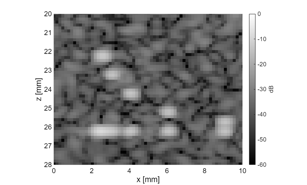
folder_path = 'figures';
mkdir(folder_path);

b_data_compare = uff.beamformed_data(img{1});
b_data_compare.data(:,1,1,1) = img{1}.data;
close all;
for i = 1:length(img)
    b_data_compare.data(:,1,1,i) = img{i}.data./max(img{i}.data);
    f = figure(i); clf;
    img{i}.plot(f, [], dynamic_range, compression);
    set(gca, 'FontSize', 18);
    xlabel('x [mm]', 'FontSize', 20); ylabel('z [mm]', 'FontSize', 20);
    colorbar off; cb = colorbar; ylabel(cb, 'dB', 'FontSize', 18);
    set(cb, 'FontSize', 16);
    % Reduce whitespace by setting paper size to match figure
    set(f, 'PaperPositionMode', 'auto');
    f.PaperUnits = 'inches';
    f.PaperPosition = [0 0 6 5];
    print(f, [folder_path, filesep, strrep(label{i}, '->', '_'), '_redone'], '-depsc2');
    axis([0 10 20 28]);
    print(f, [folder_path, filesep, strrep(label{i}, '->', '_'), '_zoomed_redone'], '-depsc2');
end

Compare beamformed data

b_data_compare.plot();

Plot timing bar chart

running_time_in_m = [time{1:5}]/60;
f99 = figure(100); clf;
bar([time{1:5}]/60);

labels_latex{1} = '$b^{\overline{T_{x DAS}}~\overline{R_{x DAS}}}$';
labels_latex{2} = '$b^{\overline{T_{x DAS}}~\overline{R_{x MV}}}$';
labels_latex{3} = '$b^{\overline{T_{x MV}}~\overline{R_{x DAS}}}$';
labels_latex{4} = '$b^{\overline{T_{x MV}}~\overline{R_{x MV}}}$';
labels_latex{5} = '$b^{\overline{R_{x MV}}~\overline{T_{x DAS}}}$';
%labels_latex{6} = '$b^{\overline{R_{x MV}}~\overline{T_{x DAS}}} \times {CF}^{0.2}$';

ylim([0 max(running_time_in_m)+1]);
ylabel('Computation time (m)');
set(gca,'FontSize',18);
x_pos = [1 2 3 4 5];
text(x_pos, running_time_in_m, num2str(running_time_in_m(:),'%.2f'), ...
    'HorizontalAlignment','center', 'VerticalAlignment','bottom', 'FontSize',18);
set(gca, 'XTickLabel', labels_latex, 'TickLabelInterpreter', 'latex', 'FontSize',24);
set(gcf,'Position',[250 344 781 470]); grid on;
saveas(f99, [folder_path, filesep, 'adaptive_timing_redone'], 'eps2c');

=========================================================================

gCNR Analysis

=========================================================================

Define ROI positions (adjust for your data!)

xc_cyst = -8e-3;       % cyst center x [m]
zc_cyst = 24.25e-3;      % cyst center z [m]
xc_speckle = -1e-3;    % speckle center x [m]
zc_speckle = 30e-3;   % speckle center z [m]
radius = 3.5e-3;      % radius [m]

% Measure gCNR for all beamformers
GCNR = zeros(1, 5);
for i = 1:5
    [~, ~, GCNR(i)] = tools.measure_contrast_circles(img{i}, xc_cyst, zc_cyst, xc_speckle, zc_speckle, radius, 0);
end

% Display results
fprintf('\n=== gCNR Comparison ===\n');
for i = 1:5
    fprintf('%-25s gCNR = %.3f\n', label{i}, GCNR(i));
end

% Plot image with ROIs indicated
f200 = figure(200); clf;
img_data = img{1}.get_image('log');
imagesc(scan.x_axis*1e3, scan.z_axis*1e3, img_data);
colormap gray; caxis([-dynamic_range 0]); axis image;
hold on;
% Draw cyst ROI (red)
theta = linspace(0, 2*pi, 100);
plot(xc_cyst*1e3 + radius*1e3*cos(theta), zc_cyst*1e3 + radius*1e3*sin(theta), 'r-', 'LineWidth', 2);
% Draw speckle ROI (green)
plot(xc_speckle*1e3 + radius*1e3*cos(theta), zc_speckle*1e3 + radius*1e3*sin(theta), 'g-', 'LineWidth', 2);
hold off;
set(gca, 'FontSize', 18);
xlabel('x [mm]', 'FontSize', 20); ylabel('z [mm]', 'FontSize', 20);
colorbar off; cb = colorbar; ylabel(cb, 'dB', 'FontSize', 18);
set(cb, 'FontSize', 16);
% Save with same settings as other images
set(f200, 'PaperPositionMode', 'auto');
f200.PaperUnits = 'inches';
f200.PaperPosition = [0 0 6 5];
print(f200, [folder_path, filesep, 'DASonRX_DASonTX_ROI_locations_redone'], '-depsc2');


% gCNR bar plot
f201 = figure(201); clf;
bar(GCNR);
xticklabels(label(1:5));
xtickangle(45);
ylabel('gCNR');
title('Generalized Contrast-to-Noise Ratio Comparison');
ylim([0 1.1]);
set(gca, 'FontSize', 14);
grid on;
% Add value labels on top of bars
x_pos = 1:5;
text(x_pos, GCNR, num2str(GCNR(:),'%.3f'), ...
    'HorizontalAlignment','center', 'VerticalAlignment','bottom', 'FontSize', 12);
saveas(f201, [folder_path, filesep, 'gCNR_res'], 'eps2c');

mean_background =

  single

    0.0615


mean_ROI =

  single

  8.4563e-04


CR =

  single

  -18.6162


CNR =

  single

    1.0911


mean_background =

    0.0476


mean_ROI =

   4.1221e-04


CR =

  -20.6271


CNR =

    1.0767


mean_background =

    0.0615


mean_ROI =

   8.4563e-04


CR =

  -18.6162


CNR =

    1.0911


mean_background =

    0.0476


mean_ROI =

   4.1221e-04


CR =

  -20.6271


CNR =

    1.0767


mean_background =

    0.0666


mean_ROI =

   7.4225e-04


CR =

  -19.5313


CNR =

    1.0922


=== gCNR Comparison ===
DASonRX->DASonTX          gCNR = 0.928
MVonRX->DASonTX           gCNR = 0.948
DASonRX->MVonTX           gCNR = 0.928
MVonRX->MVonTX            gCNR = 0.948
DASonTX->MVonRX           gCNR = 0.940

=========================================================================

FWHM / 6dB Resolution Analysis

=========================================================================

Define point target location (adjust for your data!) PICMUS numerical phantom has point targets - find the one you want to analyze

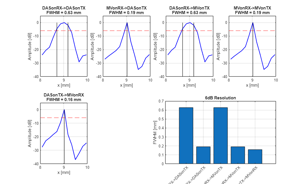
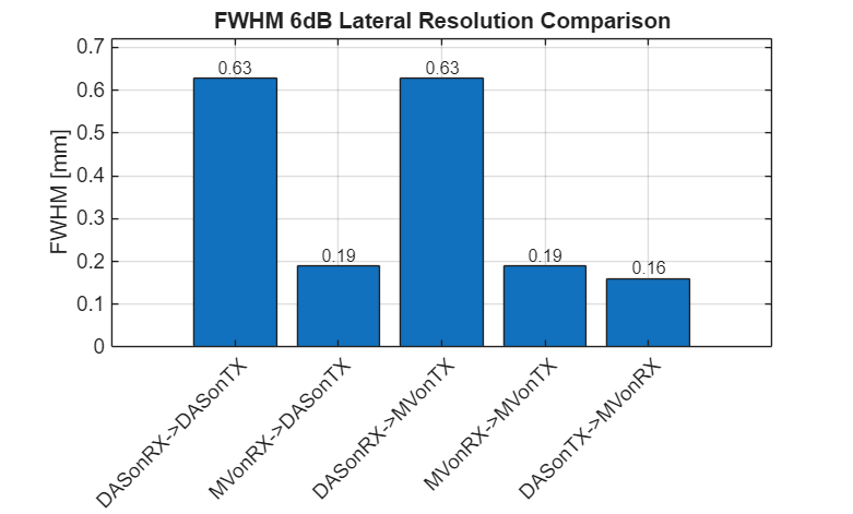
z_target = 26.2e-3;   % target depth in meters
x_target = 9e-3;      % target lateral position in meters (0 = center)
x_range = 1e-3;       % range around target to analyze [m]

% Find the z-index of the point target
[~, z_idx] = min(abs(scan.z_axis - z_target));

% Find x indices for the analysis range
x_idx_min = find(scan.x_axis >= (x_target - x_range), 1, 'first');
x_idx_max = find(scan.x_axis <= (x_target + x_range), 1, 'last');
x_range_idx = x_idx_min:x_idx_max;

% Measure FWHM for all 6 beamformers with plots
figure(300); clf;
res = zeros(1, 5);

for m = 1:5%6
    % Get lateral profile at target depth (in dB)
    img_dB = img{m}.get_image('log');
    lateral_full = img_dB(z_idx, :);

    % Extract region around target
    x_mm = scan.x_axis(x_range_idx) * 1e3;
    lateral = lateral_full(x_range_idx);
    lateral = lateral - max(lateral);  % Normalize to 0 dB at peak

    % Calculate 6dB resolution (no internal plotting)
    res(m) = compute_fwhm_6dB(x_mm, lateral);

    % Plot lateral profile
    subplot(2, 4, m);
    plot(x_mm, lateral, 'b-', 'LineWidth', 1.5);
    hold on;
    % Draw -6dB line
    yline(-6, 'r--', 'LineWidth', 1);
    % Find and mark -6dB crossing points
    idx_above = find(lateral >= -6);
    if ~isempty(idx_above)
        x_left = x_mm(idx_above(1));
        x_right = x_mm(idx_above(end));
        plot([x_left x_left], [-60 0], 'k-', 'LineWidth', 1);
        plot([x_right x_right], [-60 0], 'k-', 'LineWidth', 1);
    end
    hold off;

    xlabel('x [mm]'); ylabel('Amplitude [dB]');
    title(sprintf('%s\nFWHM = %.2f mm', label{m}, res(m)));
    ylim([-40 5]);
    grid on;
    set(gca, 'FontSize', 10);
end

% Add summary subplot
subplot(2, 4, [7 8]);
bar(res);
xticklabels(label);
xtickangle(45);
ylabel('FWHM [mm]');
title('6dB Resolution');
set(gca, 'FontSize', 10);
grid on;

% Display results
fprintf('\n=== FWHM (6dB Resolution) Comparison ===\n');
for i = 1:5
    fprintf('%-25s FWHM = %.3f mm\n', label{i}, res(i));
end

% Resolution bar plot
f301 = figure(301); clf;
bar(res);
xticklabels(label(1:5));
xtickangle(45);
ylabel('FWHM [mm]');
title('FWHM 6dB Lateral Resolution Comparison');
set(gca, 'FontSize', 14);
grid on;
set(gcf,'Position',[250 344 781 470]);
% Add value labels on top of bars
x_pos = 1:5;
text(x_pos, res, num2str(res(:),'%.2f'), ...
    'HorizontalAlignment','center', 'VerticalAlignment','bottom', 'FontSize', 12);
ylim([0 max(res)*1.15]);
saveas(f301, [folder_path, filesep, 'FWHM_res'], 'eps2c');

=========================================================================

Lateral Profile Plot

=========================================================================

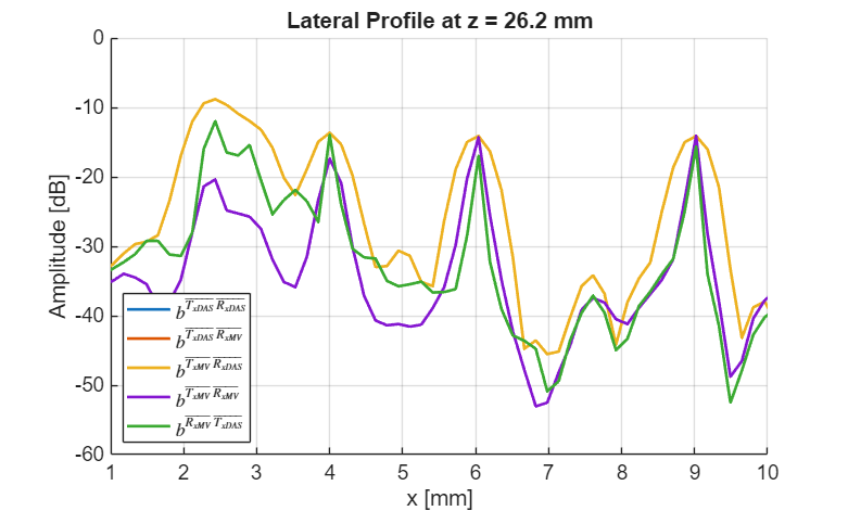
f400 = figure(400); clf;

% Get lateral profiles at target depth
colors = lines(5);
hold on;
for i = 1:5
    img_dB = img{i}.get_image('log');
    lateral = img_dB(z_idx, :);
    plot(scan.x_axis*1e3, lateral, 'LineWidth', 2, 'Color', colors(i,:));
end
hold off;

xlabel('x [mm]');
ylabel('Amplitude [dB]');
title(sprintf('Lateral Profile at z = %.1f mm', z_target*1e3));
legend(labels_latex(1:5), 'Location', 'sw', 'Interpreter', 'latex');
ylim([-dynamic_range 0]);
xlim([1 10]);
grid on;
set(gca, 'FontSize', 14);
set(gcf,'Position',[250 344 781 470]); grid on;
saveas(f400, [folder_path, filesep, 'lateral_profile_plot'], 'eps2c');

=========================================================================

Combined Bar Charts Figure

=========================================================================

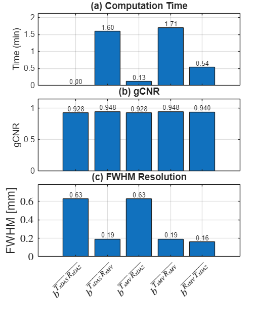
f500 = figure(500); clf;
set(gcf, 'Position', [100 100 500 650]);

% Manually position subplots for tighter layout [left bottom width height]
% Subplot 1: Computation Time (top)
ax1 = axes('Position', [0.15 0.74 0.80 0.22]);
bar(running_time_in_m);
ylabel('Time (min)');
ylim([0 max(running_time_in_m)*1.25]);
set(gca, 'FontSize', 12);
set(gca, 'XTickLabel', []);
grid on;
x_pos = 1:length(running_time_in_m);
text(x_pos, running_time_in_m, num2str(running_time_in_m(:),'%.2f'), ...
    'HorizontalAlignment','center', 'VerticalAlignment','bottom', 'FontSize', 10);
title('(a) Computation Time', 'FontSize', 14);

% Subplot 2: gCNR (middle)
ax2 = axes('Position', [0.15 0.48 0.80 0.22]);
bar(GCNR);
ylabel('gCNR');
ylim([0 1.15]);
set(gca, 'FontSize', 12);
set(gca, 'XTickLabel', []);
grid on;
x_pos = 1:5;
text(x_pos, GCNR, num2str(GCNR(:),'%.3f'), ...
    'HorizontalAlignment','center', 'VerticalAlignment','bottom', 'FontSize', 10);
title('(b) gCNR', 'FontSize', 14);

% Subplot 3: FWHM Resolution (bottom)
ax3 = axes('Position', [0.15 0.22 0.80 0.22]);
bar(res);
ylabel('FWHM [mm]');
ylim([0 max(res)*1.25]);
set(gca, 'FontSize', 12);
set(gca, 'XTickLabel', labels_latex(1:5), 'TickLabelInterpreter', 'latex', 'XTickLabelRotation', 45, 'FontSize', 16);
grid on;
x_pos = 1:5;
text(x_pos, res, num2str(res(:),'%.2f'), ...
    'HorizontalAlignment','center', 'VerticalAlignment','bottom', 'FontSize', 10);
title('(c) FWHM Resolution', 'FontSize', 14);

% Save combined figure
saveas(f500, [folder_path, filesep, 'combined_metrics_redone'], 'eps2c');

=========================================================================

Summary Table

=========================================================================

fprintf('\n=== Summary ===\n');
fprintf('%-25s %10s %10s %10s\n', 'Method', 'Time (s)', 'gCNR', 'FWHM (mm)');
fprintf('%s\n', repmat('-', 1, 60));
for i = 1:5
    fprintf('%-25s %10.2f %10.3f %10.3f\n', label{i}, time{i}, GCNR(i), res(i));
end

=== Summary ===
Method                      Time (s)       gCNR  FWHM (mm)
------------------------------------------------------------
DASonRX->DASonTX                0.12      0.928      0.627
MVonRX->DASonTX                34.92      0.948      0.190
DASonRX->MVonTX                 1.35      0.928      0.627
MVonRX->MVonTX                 34.71      0.948      0.190
DASonTX->MVonRX                11.83      0.940      0.161

=========================================================================

Local Functions

=========================================================================

function res = compute_fwhm_6dB(x_axis, y_signal)
    % COMPUTE_FWHM_6DB Compute the -6dB width (FWHM) of a signal
    %   x_axis: lateral position in mm
    %   y_signal: signal in dB (should be normalized so max = 0)
    %   res: -6dB width in mm

    % Interpolate for better resolution
    coeff = 10;
    x_interp = linspace(x_axis(1), x_axis(end), length(x_axis) * coeff);
    y_interp = interp1(x_axis, y_signal, x_interp, 'spline');

    % Find points above -6dB
    idx_above = find(y_interp >= -6);

    if isempty(idx_above)
        res = NaN;
        warning('Could not find -6dB crossing points');
        return;
    end

    % Calculate width
    res = x_interp(idx_above(end)) - x_interp(idx_above(1));
end

=== FWHM (6dB Resolution) Comparison ===
DASonRX->DASonTX          FWHM = 0.627 mm
MVonRX->DASonTX           FWHM = 0.190 mm
DASonRX->MVonTX           FWHM = 0.627 mm
MVonRX->MVonTX            FWHM = 0.190 mm
DASonTX->MVonRX           FWHM = 0.161 mm

Published with MATLAB® R2024b