DW simulation with a curvilinear array using the USTB built-in Fresnel simulator

In this example, we show how to use the built-in Fresnel simulator in USTB to generate a Focused (FI) dataset on a curvilinear array, and then beamform it with USTB.

Stefano Fiorentini stefano.fiorentini@ntu.no

20.02.2023

Contents

clear all;
close all;

Phantom

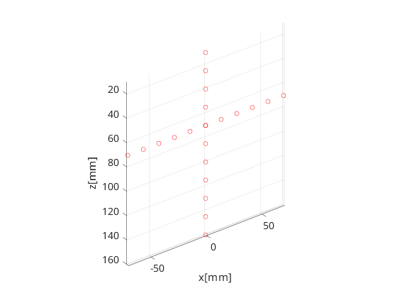
First step - define our phantom. Here, our phantom a collection of point scatterers in the shape of a cross. USTB's implementation of phantom comes with a plot method for free!

pha=uff.phantom();
pha.sound_speed=1540;            % speed of sound [m/s]
pha.points=[zeros(11,1),  zeros(11,1), linspace(10e-3,160e-3,11).', ones(11,1);...
            linspace(-70e-3,70e-3,11).',  zeros(11,1), 70e-3*ones(11,1), ones(11,1)];    % point scatterer position [m]
fig_handle=pha.plot();

Probe

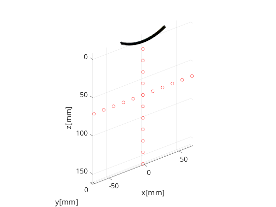
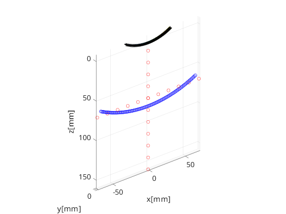
The next step is to define the probe structure which contains information about the probe's geometry. This too comes with a plot method that enables visualization of the probe with respect to the phantom. The probe we will use in our example is a curvilinear array transducer with 128 elements.

prb=uff.curvilinear_array();
prb.N=128;                  % number of elements
prb.pitch=508e-6;
prb.element_width=408e-6;
prb.radius=60e-3;
prb.plot(fig_handle);

Pulse

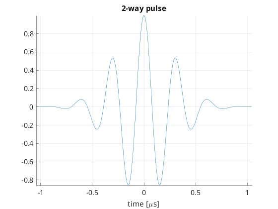
We then define the pulse-echo signal which is done here using the fresnel simulator's pulse structure. We could also use 'Field II' for a more accurate model.

pul=uff.pulse();
pul.center_frequency=3.2e6;       % transducer frequency [MHz]
pul.fractional_bandwidth=0.6;     % fractional bandwidth [unitless]
pul.plot([],'2-way pulse');

Sequence generation

Now, we shall generate our sequence! Keep in mind that the fresnel simulator takes the same sequence definition as the USTB beamformer. In UFF and USTB a sequence is defined as a collection of wave structures.

For our example here, we define a sequence of 95 focused beams. The wave structure has a plot method which plots the direction of the transmitted waves.

N=135;                             % number of focused beams
angle = linspace(-prb.maximum_angle*0.9, prb.maximum_angle*0.9, N);
focus = 0.08; % focal depth [m]

seq=uff.wave();
for n=1:N
    seq(n)=uff.wave();
    seq(n).probe=prb;
    seq(n).source.xyz=[sin(angle(n))*(prb.radius+focus), 0, cos(angle(n))*(prb.radius+focus)-prb.radius];
    seq(n).origin.xyz=[sin(angle(n))*prb.radius, 0, (cos(angle(n))-1)*prb.radius];
    seq(n).sound_speed=pha.sound_speed;

    seq(n).apodization=uff.apodization();
    seq(n).apodization.window=uff.window.rectangular;
    seq(n).apodization.f_number=5;
    seq(n).apodization.focus=uff.sector_scan('xyz',seq(n).source.xyz);

    % show source
    fig_handle=seq(n).source.plot(fig_handle);
end

The Fresnel simulator

Finally, we launch the built-in simulator. The simulator takes in a phantom, pulse, probe and a sequence of wave structures along with the desired sampling frequency, and returns a channel_data UFF structure.

sim=fresnel();

% setting input data
sim.phantom=pha;                % phantom
sim.pulse=pul;                  % transmitted pulse
sim.probe=prb;                  % probe
sim.sequence=seq;               % beam sequence
sim.sampling_frequency=40e6;  % sampling frequency [Hz]

% we launch the simulation
channel_data=sim.go();

USTB Fresnel impulse response simulator (v2.0.0)

Scan

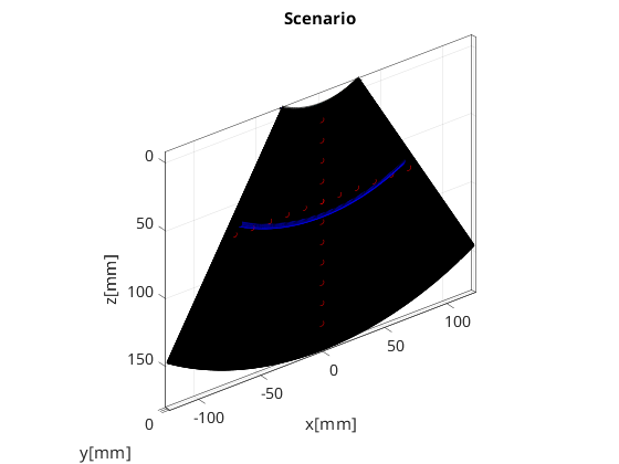
The scan area is defines as a collection of pixels spanning our region of interest. For our example here, we use the sector_scan structure, which is defined with two axes - the azimuth axis and the depth axis, along with the position of the apex. scan too has a useful plot method it can call.

scan=uff.sector_scan();
scan.azimuth_axis=linspace(-prb.maximum_angle,prb.maximum_angle,512).';
scan.depth_axis=linspace(prb.radius,prb.radius+18e-2,768).';
scan.origin=uff.point('xyz',[0 0 -prb.radius]);
scan.plot(fig_handle,'Scenario');    % show mesh

Midprocessor

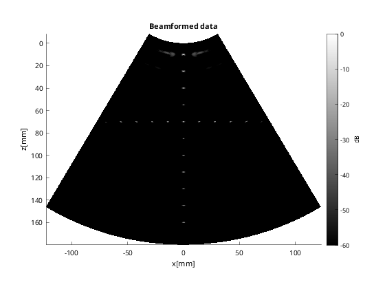
With channel_data and a scan we have all we need to produce an ultrasound image. We now use a USTB structure midprocess, that takes an apodization structure in addition to the channel_data and scan, and returns a beamformed_data.

mid=midprocess.das();
mid.dimension = dimension.both;
mid.spherical_transmit_delay_model = spherical_transmit_delay_model.unified;
mid.code = code.mex;
mid.channel_data=channel_data;
mid.scan=scan;

mid.receive_apodization.window=uff.window.hamming;
mid.receive_apodization.f_number=1.5;
mid.receive_apodization.minimum_aperture = 1e-4;
% mid.receive_apodization.maximum_aperture = 8e-2;

mid.transmit_apodization.window=uff.window.hamming;
mid.transmit_apodization.f_number=3.5;
mid.transmit_apodization.minimum_aperture = 4e-3;
% mid.transmit_apodization.maximum_aperture = 2e-2;

% beamforming
b_data=mid.go();
b_data.plot();

USTB MEX C beamformer...Completed in 8.51 seconds.

Published with MATLAB® R2024b