Contrast of Delay Multiply And Sum on FI data from an UFF file

by Ole Marius Hoel Rindal olemarius@olemarius.net

Last updated 07.08.2017

Setting up file path
Reading channel data from UFF file
Define Scan
Set up the processing pipeline
Define the DAS beamformer
Create the DMAS image using the delay_multiply_and_sum postprocess
Beamform DAS image
Plot both images in same plot
Measure contrast

Setting up file path

To read data from a UFF file the first we need is, you guessed it, a UFF file. We check if it is on the current path and download it from the USTB websever.

clear all; close all;

% data location
url = tools.zenodo_dataset_files_base();
local_path = [ustb_path(),'/data/']; % location of example data

% Choose dataset
filename='Alpinion_L3-8_FI_hypoechoic.uff';

% check if the file is available in the local path or downloads otherwise
tools.download(filename, url, local_path);

Reading channel data from UFF file

channel_data=uff.read_object([local_path filename],'/channel_data');
% Check that the user have the correct version of the dataset
if(strcmp(channel_data.version{1},'1.0.2')~=1)
    error(['Wrong version of the dataset. Please delete ',local_path,...
                                        filename,' and rerun script.']);
end

UFF: reading channel_data [uff.channel_data]
UFF: reading sequence [uff.wave] [====================] 100%

%Print info about the dataset
channel_data.print_authorship

Name: 		 FI dataset of hypoechic cyst recorded on an  
		 Alpinion scanner with a L3-8 Probe from a CIRC  
		 General Purpose Ultrasound Phantom 
Reference: 	 www.ultrasoundtoolbox.com 
Author(s): 	 Ole Marius Hoel Rindal <olemarius@olemarius.net> 
		 Muyinatu Lediju Bell <mledijubell@jhu.edu> 
Version: 	 1.0.2

Define Scan

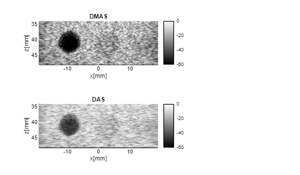
Define the image coordinates we want to beamform in the scan object. Notice that we need to use quite a lot of samples in the z-direction. This is because the DMAS creates an "artificial" second harmonic signal, so we need high enough sampling frequency in the image to get a second harmonic signal.

z_axis=linspace(34e-3,48e-3,750).';
x_axis=zeros(channel_data.N_waves,1);
for n=1:channel_data.N_waves
    x_axis(n) = channel_data.sequence(n).source.x;
end

scan=uff.linear_scan('x_axis',x_axis,'z_axis',z_axis);

Set up the processing pipeline

pipe=pipeline();
pipe.channel_data=channel_data;
pipe.scan=scan;

pipe.transmit_apodization.window=uff.window.scanline;

pipe.receive_apodization.window=uff.window.none;
pipe.receive_apodization.f_number=1.7;

Define the DAS beamformer

das = midprocess.das();
%Sum only on transmit, so that we can do DMAS on receice
das.dimension = dimension.transmit();

Create the DMAS image using the delay_multiply_and_sum postprocess

dmas = postprocess.delay_multiply_and_sum();
dmas.dimension = dimension.receive;
dmas.channel_data = channel_data;
dmas.receive_apodization = pipe.receive_apodization;

b_data_dmas=pipe.go({das dmas});

% beamforming
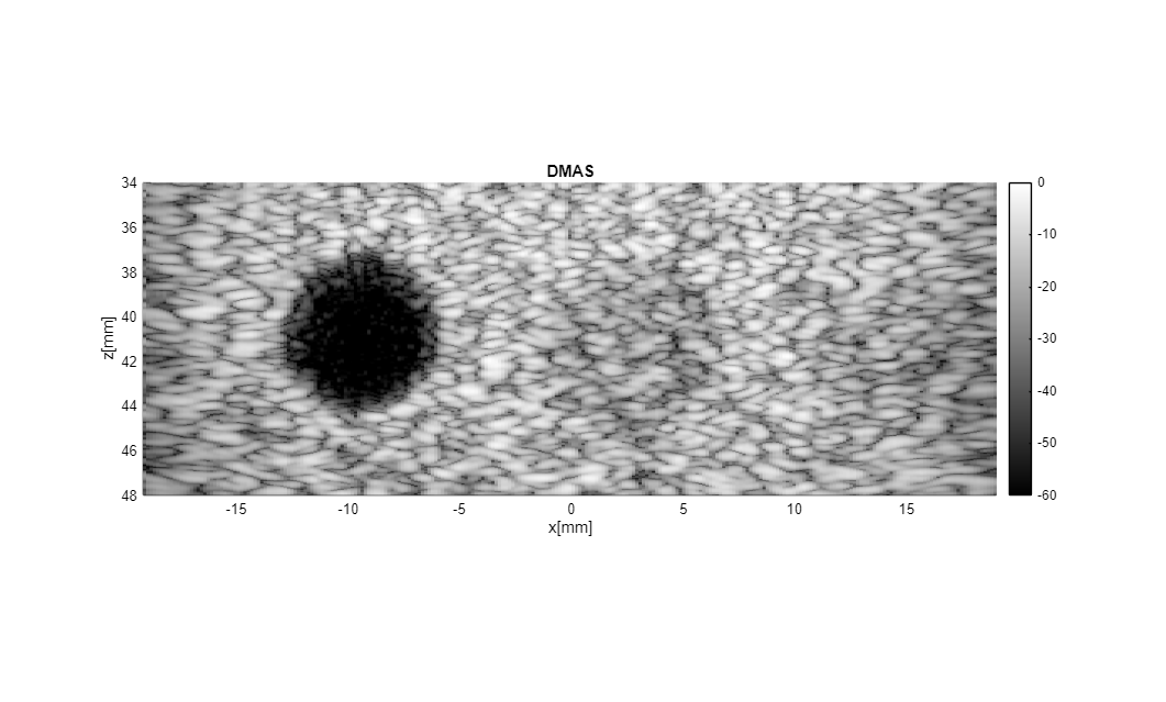
b_data_dmas.plot(100,'DMAS');

USTB MEX C beamformer...Completed in 0.12 seconds.

f_stop =

  single

    10779359

Warning: If the result looks funky, you might need to tune the filter paramters
of DMAS using the filter_freqs property. Use the plot to check that everything
is OK.

Beamform DAS image

Notice that I redefine the beamformer to use Hamming apodization and summing on both transmit and receive.

das.dimension = dimension.both();
das.receive_apodization.window=uff.window.hamming;
das.receive_apodization.f_number=1.7;

b_data_das=pipe.go({das});
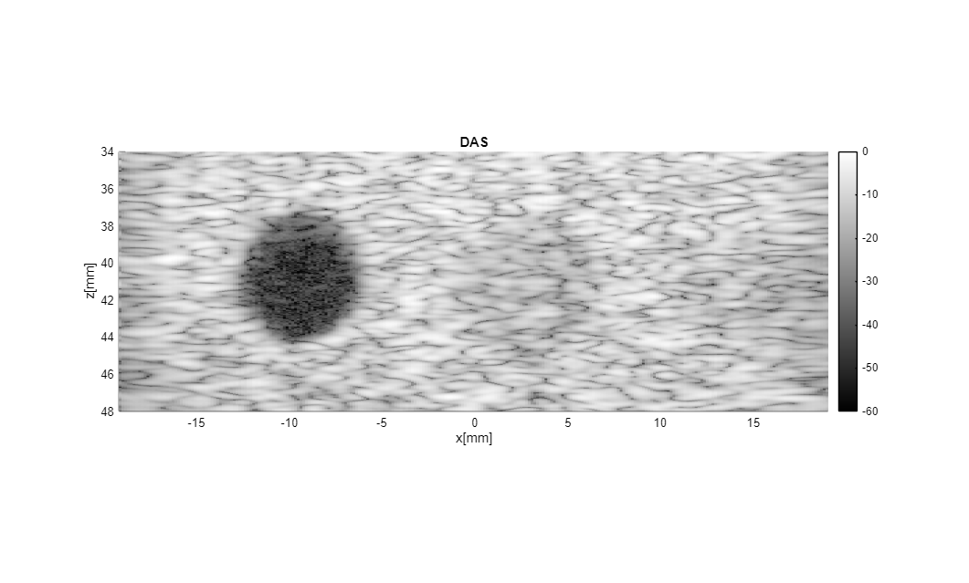
b_data_das.plot([],'DAS');

USTB MEX C beamformer...Completed in 0.06 seconds.

Plot both images in same plot

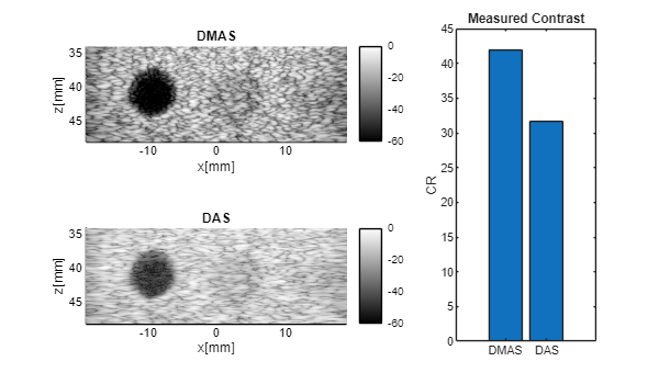
Plot both in same plot with connected axes, try to zoom!

f3 = figure(3);clf
set(f3,'Position',[200,200,600,350])
b_data_dmas.plot(subplot(2,3,[1 2]),'DMAS'); % Display image
ax(1) = gca;
b_data_das.plot(subplot(2,3,[4 5]),'DAS'); % Display image
ax(2) = gca;
linkaxes(ax);

Measure contrast

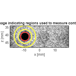
Lets measure the contrast using the "contrast ratio" as our metric.

% First we need to put our images in a different data struct that the
% measure contrast function expects
images.all{1} = b_data_dmas.get_image();
images.all{2} = b_data_das.get_image();

% Define the coordinates of the regions used to measure contrast
xc_nonecho = -9.5;      % Center of cyst in X
zc_nonecho = 40.8;      % Center of cyst in Z
r_nonecho = 2.8;        % Radi of the circle in the cyst
r_speckle_inner = 4.5;  % Radi of the inner circle defining speckle region
r_speckle_outer = 7;    % Radi of the outer circle defining speckle region

% Call the "tool" to measure the contrast
[CR] = tools.measure_contrast_ratio(b_data_das,images,xc_nonecho,...
                    zc_nonecho,r_nonecho,r_speckle_inner,r_speckle_outer);

% Plot the contrast as a bar graph together with the two images
figure(3);hold on
subplot(2,3,[3 6]);
bar(CR)
set(gca,'XTickLabel',{'DMAS','DAS'})
title('Measured Contrast');
ylabel('CR');