Demonstrating Fourier beamforming on STAI data

This script implements and compares three ultrasound beamforming methods:
 1. Wavenumber Algorithm (WA)
 2. DAS-Consistent Wavenumber (DCWA)
 3. Delay-and-Sum (DAS)

For details, see: - S. Mulani, M. S. Ziksari, A. Austeng and S. P. Näsholm,
"Delay-and-Sum Consistent Wavenumber Algorithm," in IEEE Transactions on
Ultrasonics, doi: 10.1109/TUSON.2026.3667456.

Author:    Sufayan Mulani <sufayanm@uio.no>

Contents

Download and load channel data (UFF format)

The dataset is downloaded from Zenodo

fn = 'STAI_UFF_CIRS_phantom.uff';
local_path = [ustb_path(), '/data/'];
url = tools.zenodo_record_files_base('19860810');
tools.download(fn, url, local_path);
uff_file = fullfile(local_path, fn);
channel_data = uff.read_object(uff_file, '/channel_data');

UFF: reading channel_data [uff.channel_data]
UFF: reading sequence [uff.wave] [====================] 100%

Define reconstruction scan grid

scan=uff.linear_scan('x_axis', linspace(-20e-3, 20e-3, 512).', 'z_axis', linspace(10e-3, 80e-3, 512).');

Demodulate RF channel data to baseband (IQ) data

demod = preprocess.demodulation();
demod.input = channel_data;
channel_data_demod = demod.go();

Warning: The modulation frequency is not specified. The estimated central
frequency will be used.  
Estimating power spectrum
Warning: The downsampling frequency is not specified. Using 2 *
modulation_frequency. 
Warning: The input sample frequency is not a multiple of the specified
downsample frequency. Rounding up the downsample frequency to the next higher
downsample frequency. 
Band-pass filtering
Low-pass filtering

Wavenumber algorithm (WA)

mid = midprocess.Fourier_beamforming ;
mid.channel_data  = channel_data_demod ;
mid.scan          = scan ;
mid.spatial_padding = 2 ;     % Improves interpolation accuracy
mid.temporal_padding = 2 ;    % Improves interpolation accuracy
mid.DAS_consistent = false ;  % Flag indicating DCWA mode
mid.USTB_scan = false ;       % Keep reconstruction grid defined in the algorithm
mid.temp_origin = 40e-3 ;     % Shifts temporal origin to the defined depth [m]
mid.angle_apodization = 30 ;  % Angular cutoff [deg]
% Beamforming
w_data = mid.go() ;
% Display result
% w_data.plot([], w_data.name, []) ;

% Normalize image
wavenumber_image = w_data.get_image('abs') ;
wavenumber_image = wavenumber_image/max(wavenumber_image(:)) ;

Number of samples in data - 1344 
Number of samples in zero-padded data - 2774 

Interpolating frame no - 256 / 256
Elasped time for WA is 19.05 seconds. 

DAS consistent wavenumber algorithm (DCWA)

mid = midprocess.Fourier_beamforming ;
mid.channel_data  = channel_data_demod ;
mid.scan          = scan ;
mid.spatial_padding = 2 ;     % Improves interpolation accuracy
mid.temporal_padding = 2 ;    % Improves interpolation accuracy
mid.DAS_consistent = true ;   % Flag indicating DCWA mode
mid.USTB_scan = false ;       % Keep reconstruction grid defined in the algorithm
mid.temp_origin = 40e-3 ;     % Shifts temporal origin to the defined depth [m]
mid.angle_apodization = 30 ;  % Angular cutoff [deg]
% Beamforming
DCWA_data = mid.go() ;
% Display result
% DCWA_data.plot([], DCWA_data.name, []) ;

% Normalize image
DCWA_image = DCWA_data.get_image('abs') ;
DCWA_image = DCWA_image/max(DCWA_image(:)) ;

Number of samples in data - 1344 
Number of samples in zero-padded data - 2774 

Interpolating frame no - 256 / 256
Elasped time for DCWA is 17.54 seconds. 

DAS method

mid = midprocess.das ;
mid.channel_data=channel_data_demod;
mid.scan = w_data.scan;
apod_angle = 30 ;            % Angular cutoff [deg]
f_number = cot(deg2rad(apod_angle))/2 ;

% Transmit apodization
mid.transmit_apodization.f_number = f_number ;
mid.transmit_apodization.window = uff.window.tukey25 ;
mid.transmit_apodization.minimum_aperture = [0 0] ;
mid.transmit_apodization.maximum_aperture = [1e5 1e5] ;

% Receive apodization
mid.receive_apodization.f_number = f_number ;
mid.receive_apodization.window = uff.window.tukey25 ;
mid.receive_apodization.minimum_aperture = [0 0] ;
mid.receive_apodization.maximum_aperture = [1e5 1e5] ;

% Beamforming
b_data=mid.go() ;
% Display result
% b_data.plot([],'DAS',[] );

% Normalize image
das_image = b_data.get_image('abs') ;
das_image = das_image/max(das_image(:)) ;

USTB MEX C beamformer...Completed in 17.81 seconds.

Image comparison

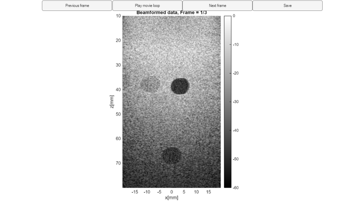
b_data_compare = uff.beamformed_data(w_data)
b_data_compare.data(:,:,1) = w_data.data;
b_data_compare.data(:,:,2) = DCWA_data.data;
b_data_compare.data(:,:,3) = b_data.data;
b_data_compare.plot()

b_data_compare = 

  beamformed_data with properties:

                    scan: [1×1 uff.linear_scan]
                    data: [255012×1 single]
                 phantom: []
                sequence: []
                   probe: []
                   pulse: []
      sampling_frequency: []
    modulation_frequency: []
              frame_rate: 1
                N_pixels: 255012
              N_channels: 1
                 N_waves: 1
                N_frames: 1
                    name: 'WA'
               reference: {}
                  author: {}
                 version: {}
                    info: {}


ans = 

  Figure (1) with properties:

      Number: 1
        Name: ''
       Color: [1 1 1]
    Position: [323 225 1061 639]
       Units: 'pixels'

  Use GET to show all properties

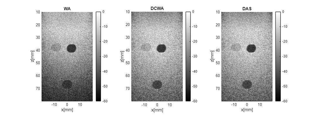
figure
set(gcf, "Position", [0.1818    0.3994    1.0904    0.4008]*1e3)
w_data.plot(subplot(1,3,1), "WA") ;
DCWA_data.plot(subplot(1,3,2), "DCWA") ;
b_data.plot(subplot(1,3,3), "DAS") ;

Legends for plots

legends_(1) = "WA" ;
legends_(2) = "DAS" ;
legends_(3) = "DCWA" ;

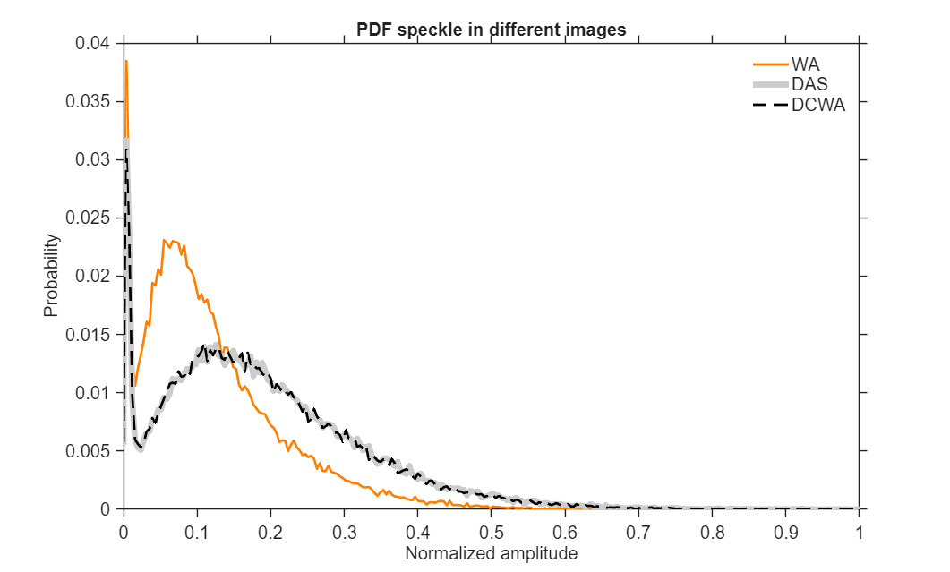
Probability distribution function (PDF) of speckle

scan_ = w_data.scan ;

% Region of interest for speckle analysis
X_lim = [-15, 11] ;    % [mm]
Y_lim = [29, 49] ;     % [mm]

x_lim_points = get_index(X_lim, 1e3*scan_.x_axis, 1) ;
y_lim_points = get_index(Y_lim, 1e3*scan_.z_axis, 1) ;

% Compute histograms
[das_hist, das_edge] = imhist(das_image(y_lim_points(1):y_lim_points(2), x_lim_points(1):x_lim_points(2))) ;
[wavenumber_hist, wavenumber_edge] = imhist(wavenumber_image(y_lim_points(1):y_lim_points(2), x_lim_points(1):x_lim_points(2))) ;
[dcwa_hist, dcwa_edge] = imhist(DCWA_image(y_lim_points(1):y_lim_points(2), x_lim_points(1):x_lim_points(2))) ;

% Normalize to get probability distributions
das_hist = das_hist/sum(das_hist) ;
wavenumber_hist =wavenumber_hist/sum(wavenumber_hist) ;
dcwa_hist = dcwa_hist/sum(dcwa_hist) ;

figure
plot(wavenumber_edge, wavenumber_hist, LineWidth=2, DisplayName="WA with TGC", Color=[255 128 0]/255)
hold on
plot(das_edge, das_hist, LineWidth=5, DisplayName=legends_(2), Color=0.8*[1 1 1])
plot(dcwa_edge, dcwa_hist, LineWidth=2, DisplayName=legends_(3), LineStyle="--", Color='k')

legend(legends_, Box="off")
xlabel('Normalized amplitude')
ylabel('Probability')
title('PDF speckle in different images')
fontsize(gcf, 15, 'points')
set(gca, "TickDir", "out")

PDF of the difference between images reconstructed using DAS, DCWA and WA

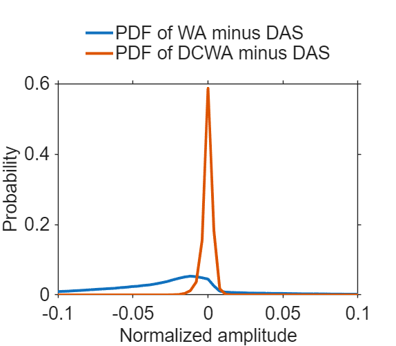
% Region of interest
Y_lim = [20 80] ;   % [mm]
X_lim = [-18 18] ;  % [mm]

edges_ = linspace(-1, 1, 513) ;   % Histogram bin edges

% Compute pixel-wise difference images
diff_wa_das = wavenumber_image-das_image ;
diff_dcwa_das = DCWA_image-das_image ;

x_lim_points = get_index(X_lim, 1e3*scan_.x_axis) ;
y_lim_points = get_index(Y_lim, 1e3*scan_.z_axis, 1) ;

% Compute histograms of the differences
[f_das_hist, f_das_edge] = histcounts(diff_dcwa_das(y_lim_points(1):y_lim_points(2), x_lim_points(1):x_lim_points(2)), edges_) ;
[wavenumber_hist, wavenumber_edge] = histcounts(diff_wa_das(y_lim_points(1):y_lim_points(2), x_lim_points(1):x_lim_points(2)), edges_) ;

% Normalize to obtain probability distributions
f_das_hist = f_das_hist/sum(f_das_hist) ;
wavenumber_hist =wavenumber_hist/sum(wavenumber_hist) ;

% Plot the difference PDFs
figure
plot(wavenumber_edge(2:end), (wavenumber_hist), LineWidth=3, DisplayName="PDF of WA minus DAS")
hold on
plot(f_das_edge(2:end), (f_das_hist) ,LineWidth=3, DisplayName="PDF of DCWA minus DAS")

legend("Location","northoutside", "Box","off")
xlim([-0.1 0.1])
xlabel('Normalized amplitude')
ylabel('Probability')
fontsize(gcf, 20, 'points')
set(gca, "TickDir", "out")
set(gcf, "Position", [0.3514    0.3298    0.5736    0.5000]*1e3)

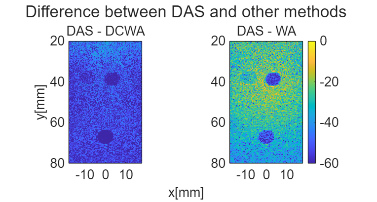
Display difference between images

The differences are shown in dB;

figure
t2 = tiledlayout(1,2,'TileSpacing','Compact','Padding','Compact');

% DAS vs DCWA
nexttile
imagesc(scan_.x_axis*1e3, scan_.z_axis*1e3, db(DCWA_image-das_image), [-60, 0])
title("DAS - DCWA", 'FontWeight','normal')
axis tight equal
ylim(Y_lim)
xlim(X_lim)

% DAS vs WA
nexttile
imagesc(scan_.x_axis*1e3, scan_.z_axis*1e3, db(wavenumber_image-das_image), [-60, 0])
title("DAS - WA", 'FontWeight','normal')
axis tight equal
ylim(Y_lim)
xlim(X_lim)
colorbar

fontsize(20,'points')
xlabel(t2, 'x[mm]')
ylabel(t2, 'y[mm]') ;
title(t2, "Difference between DAS and other methods", 'fontsize', 25 )
set(gcf, "Position", [132  437  764  409])

Maximum value of the difference images

diff_wa_das = db(wavenumber_image-das_image);
diff_dcwa_das = db(DCWA_image-das_image) ;
fprintf(['The maximum of the difference between DAS and WA is %4.4f dB \nand' ...
    ' the maximum of the difference between DAS and DAS-Fourier is %4.4f dB' ...
    ' \n'], max(diff_wa_das(:)), max(diff_dcwa_das(:)))

The maximum of the difference between DAS and WA is -5.4495 dB 
and the maximum of the difference between DAS and DAS-Fourier is -30.3550 dB 

Quantitative metrics: SSIM and MSE

SSIM (Structural Similarity Index) - closer to 1 means more similar MSE (Mean Squared Error) - closer to 0 means more similar

fprintf("SSIM (WA vs DAS): %0.4f \n", ssim(single(wavenumber_image), das_image))
fprintf("SSIM (DCWA vs DAS): %0.4f \n", ssim(single(DCWA_image), das_image))
fprintf("MSE (WA vs DAS): %0.4f \n", immse(single(wavenumber_image), das_image) )
fprintf("MSE (DCWA vs DAS): %0.4f \n", immse(single(DCWA_image), das_image) )

SSIM (WA vs DAS): 0.6257 
SSIM (DCWA vs DAS): 0.9978 
MSE (WA vs DAS): 0.0050 
MSE (DCWA vs DAS): 0.0000 

Vertical line profile from the reconstructed images

Lat_dist = 0e-3 ;       % Lateral position of line (m)
lat_index = get_index(Lat_dist, scan_.x_axis);
Thickness_lat = 0e-3 ;  % Lateral averaging thickness (m)
Thickness_index = round(Thickness_lat/scan_.x_step) ;

Full_image = cat(3, db(wavenumber_image), db(das_image), db(DCWA_image));

temp_mat = Full_image(:, lat_index-Thickness_index:lat_index+Thickness_index, :) ;
temp_mat(temp_mat<-100) = -100 ;   % Clip extreme low values for stability
vert_plot = squeeze(max(temp_mat, [], 2)) ;

% Resample on a denser axial grid using spline interpolation for smoother curves
dense_z_axis = linspace(min(scan_.z_axis), max(scan_.z_axis), scan_.N_z_axis) ;
dense_vert_plot = interp1(scan_.z_axis, vert_plot, dense_z_axis, "spline", 0) ;
dense_vert_plot = dense_vert_plot - max(dense_vert_plot, [], 1) ;

% Plot axial profiles for each method
figure;
plot(dense_z_axis*1e3, dense_vert_plot(:,1), LineWidth=2, DisplayName=legends_(1) )
hold on
plot(dense_z_axis*1e3, dense_vert_plot(:, 2), LineWidth=5, DisplayName=legends_(2), Color=0.8*[1 1 1])
hold on
plot(dense_z_axis*1e3, dense_vert_plot(:,3), LineWidth=2, DisplayName=legends_(3), LineStyle="--", Color='k')

xlabel('Axial Distance [mm]')
ylabel('Amplitude [dB]')
le = legend(Location="southeast") ;
le.Position = [0.4513    0.1482    0.4345    0.2130] ;
legend(Box="off")
xlim([40.77 50.77])
ylim([-40 -4])
set(gca, "FontSize", 15)

This function finds the index of closest number to 'dist' in 'in_axis'

function out_index = get_index(dist, in_axis, out_range)
if nargin<3
    out_range = 0;
end
if isscalar(dist)
    if dist>max(in_axis)||dist<min(in_axis)
        if out_range==0
            error("Querry value is not in the range of sample points")
        end
    end
    [~, out_index] = min(abs(dist - in_axis(:))) ;
else
    size_dist = size(dist) ;
    dist = reshape(dist, 1, []) ;
    in_axis = in_axis(:) ;
    if max(dist)>max(in_axis)||min(dist)<min(in_axis)
        if out_range==0
            error("Some of the querry values are not in the range of sample points. " + ...
                "If you want to proceed anyway use 1 as a third argument while calling the function")
        end
    end
    [~, out_index] = min(abs(dist - in_axis)) ;
    out_index =  out_index(:) ;
    out_index = reshape(out_index, size_dist) ;
end
end

Published with MATLAB® R2025a